UMich’s Index of Deep Disadvantage shows that the highest concentrations of deep disadvantage are often rural and clustered in the Mississippi Desslta and Cotton Belt, across much of Appalachia, along the Texas‑Mexico border, in several Rust Belt cities, and on Tribal Nation lands.
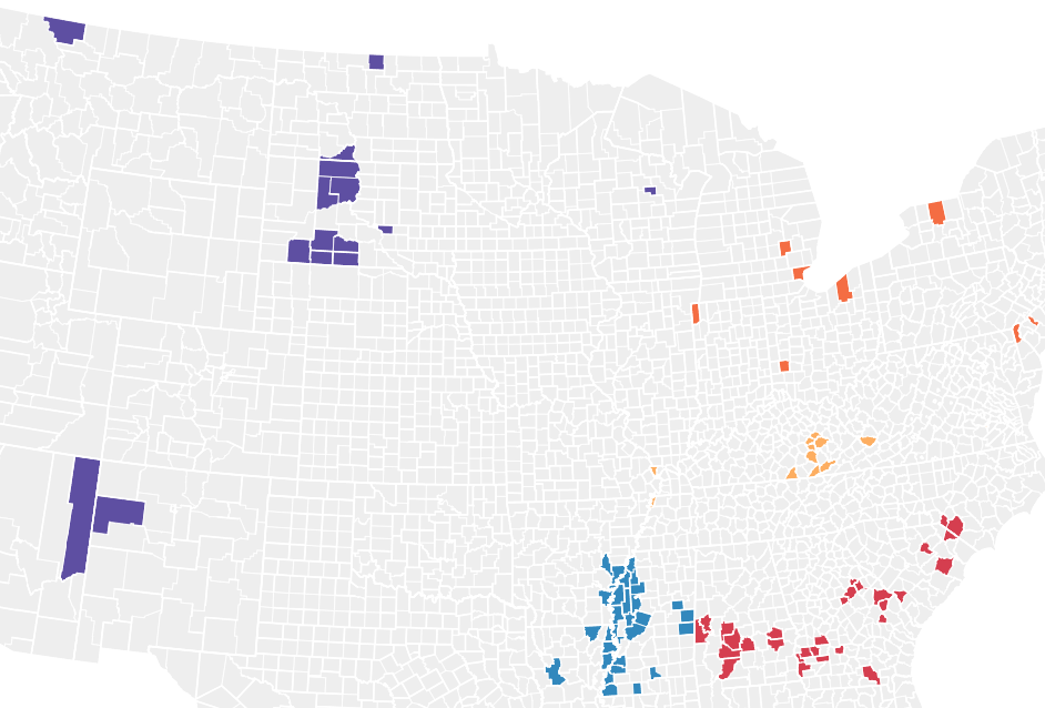
Understanding these clusters of deep poverty helps us anticipate both assets and constraints — factors such as like anchor employers, hospital access, and historical barriers that shape today’s economic environment.
The Index of Deep Disadvantage is multidimensional, blending three domains:
- Income – both poverty and deep poverty rates
- Poverty is defined as the share of community residents whose pre‑tax cash income falls below the federal poverty threshold for their family size and ages. Thresholds are set nationally, not locally, and updated each year using the Consumer Price Index.
- Deep, or “Extreme Poverty” is defined as the share of community residents whose pre‑tax cash income falls below half of the poverty threshold for their family size and ages. (This excludes noncash benefits, like SNAP or housing vouchers, and does not count tax credits like the EITC.)
- Health – life expectancy and low birthweight
- Mobility – intergenerational economic mobility estimates (from Opportunity Insights)
The IDD research team standardizes those variables and has used principal component analysis to create a composite index and rank places on a relative scale of disadvantage. This gives us a holistic, county‑comparable measure rather than a single‑issue snapshot.
- Rural overrepresentation – Of the 100 most disadvantaged places, the overwhelming majority are rural. This matters because rural areas generally have thinner services, longer distances, and lower tax bases — all factors that influence how far a cash can travel and how much local capacity, if any, there is to amplify the cash.
- Severe outcome gaps – In the most disadvantaged communities, average life expectancy is nearly a decade shorter than in the most advantaged communities. Disparities in poverty and deep poverty are stark. Those are structural signals about the local opportunity environment — the very conditions cash must contend with.
- Place (and history) matters – The clustering patterns mirror legacies of exploitation and disinvestment. The index surfaces the history of slavery or relocation in today’s data, reminding us to design with local context, not just statistics.
Success on a County Level
- Household mobility – Increased employment stability, credential attainment, childcare continuity, and reduced debt in participating households.
- Market response – Noticeable spending at local businesses, reduced rental arrears, improved utility payment rates — signals that dollars are circulating locally.
- System leverage – County partners using RGMII data to simplify benefits navigation, extend clinic hours, or adjust local grantmaking.
- Narrative shift – Rural residents’ own stories leading the case for scaling guaranteed income, grounded in local realities (see our program pages for how we publish these stories ethically and securely) such as those in the OpenResearch Study Analysis
Conclusion
The University of Michigan’s Index of Deep Disadvantage names and locates rural disadvantage more rigorously, moving us beyond anecdotes to a shared map. Second, it highlights mobility – the county‑level spark that allows guaranteed income to go beyond immediate relief toward genuine opportunity.
With humility about what cash can and cannot do on its own, we can direct resources where can potentially have the greatest effect – counties where new prosperity can spread and help nearby counties in the deepest disadvantage. With your help, we hope to slowly widen the impact of Guaranteed Minimum Income, county by county, state by state, throughout America.
References
- Poverty Solutions at the University of Michigan. Index of Deep Disadvantage—Final Data. Google Sheets, 2020. Accessed September 11, 2025.
- Poverty Solutions at the University of Michigan, and Center for Research on Child Wellbeing, Princeton University. “Index of Deep Disadvantage: Technical Documentation.” 2020. Accessed September 11, 2025.
- Poverty Solutions at the University of Michigan. “Understanding Communities of Deep Disadvantage.” Poverty Solutions (project overview and data tools), 2020. Accessed September 11, 2025. .
- Shaefer, H. Luke, Kathryn Edin, and Tim Nelson. Understanding Communities of Deep Disadvantage: An Introduction. Ann Arbor, MI: Poverty Solutions, University of Michigan; Princeton, NJ: Center for Research on Child Wellbeing, Princeton University, January 29, 2020.
- Wadley, Jared. “New Index Ranks America’s 100 Most Disadvantaged Communities.” University of Michigan News, January 30, 2020. Accessed September 11, 2025.